By Timothy W. Thomas
North Rose-Wolcott High School
Earth Science
REM-SMT Project 2003-04
List of Topics:
I. Introduction
II. Scope of Project
II. Scope of Project
III. Temperature Analysis
IV. Dew Point Analysis
V. Conclusion
VI. Topics for Further Research
I. Introduction
I. Introduction
In the field of Meteorology, forecasters often use computer models to aid in the formation of their forecasts on a daily, and even in some cases hourly, basis. As these computer models become more accurate, meteorologists’ forecasts will inherently become more accurate as well. This can lead to greater lead times on storm warnings, greater preparation time for extreme weather, and higher ratings for on-air meteorologists.
One of these models is the Mesoscale Meteorological Model Version 5.0 (MM5). This model has a small grid spacing of approximately 6 miles and generates forecasts out to 36 hours from initialization. With its relatively short forecast timeframe and small grid spacing, it has the potential to not only forecast synoptic events, but also smaller mesoscale events like thunderstorm initiation, sea-breeze generation, and lake effect snow events to a potentially higher degree of accuracy than the large scale models (ETA, NGM, etc.). To test MM5’s accuracy, with the help of the Meteorology staff at SUNY Oswego, forecasts have been generated using the MM5 model configured for the North Rose-Wolcott High School location during the month of February 2004, where a Davis Vantage PRO wireless weather station has been installed (Diagrams 1-a, 1-b).
II. Scope of Project
II. Scope of Project
This project has focused on the accuracy of the MM5 model forecasts for temperature and dew point temperature for the NR-W High School location during the month of February 2004. MM5 model forecasts (00Z-36Z) for these two parameters initialized at 00Z were analyzed. Using Excel spreadsheets, the hourly model forecasts have been collected every day (available on the data disc or upon request), along with the verification (or real) readings recorded by VORTEX (see Table A).
The statistical analysis includes graphical representations of actual and average hourly and daily errors, average forecast hour summary errors, daily standard deviations, and daily average error. From the graphs generated, trends in the data are outlined and discussed, including any warm or cold bias. Error have been determined by taking the difference between the forecast value and the recorded value by VORTEX, which is a 30-minute average. Since VORTEX records on a 30 minute cycle, in order to match up these values with the MM5 forecast values, we had to take every other value (those recorded on the hour).
III. Temperature
III. Temperature
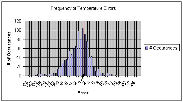
When looking at the plots associated with temperature, several interesting trends can be noticed. The most pronounced is an overall cold bias in the MM5 forecasts shown by graphs #1 and #2. Graph #1 shows the frequency of absolute errors over the course of the entire month of February. The arrow and red line in the center of the graph indicates the zero mark. Since there
Graph #1
is a greater majority of the values in the negative region, we can conclude that the model had a cold bias for the month in terms of temperature. However, it is also important to note that the overall majority of the values are close to zero (+2 to -2) indicating a fair amount of accuracy, despite the cold bias. Graph #2 shows the average temperature error for each forecast hour
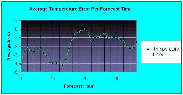
Graph #2
from initialization through the 36-hr. forecast. Again one can see an obvious cold bias, particularly for the 6Z through 15Z forecasts. This would suggest that the model generally forecasts colder temperatures during the overnight hours, and only slightly colder during the daytime hours on average.
Along with the monthly and hourly totals, graphs have been produced for each day to see if there are any daily fluctuations or any extreme cases. On most of the daily graphs, the errors tend to fluctuate from slightly warmer to slightly cooler with no sudden jumps and most tend to range from –10 to +10 from the verification. Graph #3 shows the average error for the entire forecast each day throughout February. Again, one can see that more values are below zero, indicating the cold bias. An interesting feature on this graph, is the apparent oscillation in the values from the beginning of the month right through to the end. This could be an area for further research, either at finding the reason(s) behind the oscillation and/or comparing this month to other months to see if the same patterns occur.
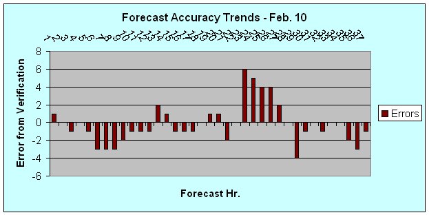
While most values range from +10 to –10, there are a few days when the model was significantly off in the temperature forecast (February 6th and 10th). The most significant in this study was February 10th (Graph #4), where the entire forecast was colder than what verified (average of –12.4 degrees Fahrenheit), and the 08Z through 10Z forecasts were 20 degrees colder than the verification. February 6th had a significant error as well (average of –12.8 degrees
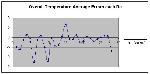
Graph #3
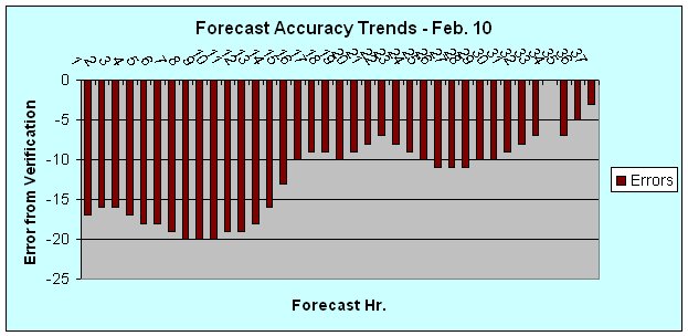
Graph #4
Fahrenheit), however there are data gaps for the 6th yielding some uncertainty to the extent of the negative error. A possible explanation for the extreme cold bias could be an error in the timing of a cold front. For instance, if the model forecast the passage of the cold front too soon, this would result in colder forecast temperatures, and vice-versa if a warm bias was observed.
Lastly, Graph #5 shows the overall standard deviations for each day. In general, this parameter ranges from 2 to 5, with the exception of February 14th where the standard deviation was 7. Again, one can notice an apparent oscillation throughout the month that does not match up with the same oscillating pattern observed on graph #4.
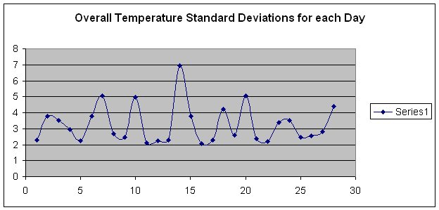
Graph #5
IV. Dew Point
IV. Dew Point
The dew point plots also reveal some interesting trends. The plot showing the average forecast error per forecast period (Graph #6) indicates a diurnal trend: during the late night and into the early morning hours (00Z through 10Z) the model forecasts for too much moisture, while during the late morning into the afternoon (12Z through 20Z) it under-forecasts the moisture content of the air, and then overnight (23Z through 36Z) it again forecasts too much moisture. This could be attributed to the close proximity of the High School to Lake Ontario (approximately 6 miles), but since the grid spacing for the model is 6 miles, the lake is not likely to be in the domain of the grid. A slight warm bias is also observed.
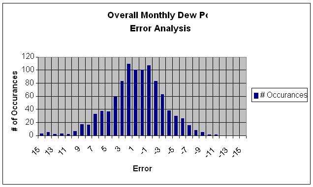
The plot of overall monthly errors (Graph #7) shows only a slight warm bias, indicating a small trend to forecast for a slightly higher moisture content. The daily forecast errors were also fairly uniform and evenly distributed. Looking at February 10th, since the forecast temperatures were off quite a bit, one can notice that the model did a good job at forecasting the dew point temperatures during the same time period. This may eliminate the possibility of forecasting the
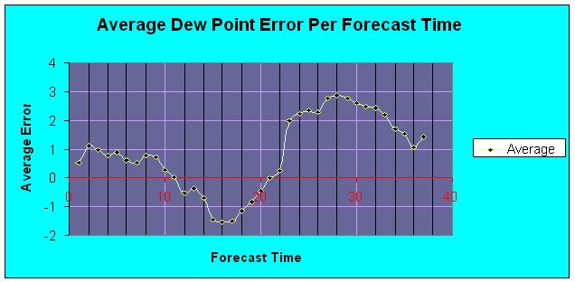 Graph #6
Graph #7
Graph #8
timing a frontal passage poorly, since the air behind a cold front is generally drier. Had the model forecast an early passage of the front, not only would we expect to see a cold bias in the temperature forecast, but we would expect to find a cold bias in the dew points as well.
Graphing the overall standard deviations for each day reveals a similar oscillating/cyclic trend to those observed in the temperature standard deviation plot. The only difference is that the values tend to fluctuate at a higher frequency for dew point (Graph #9). Likewise, we also see
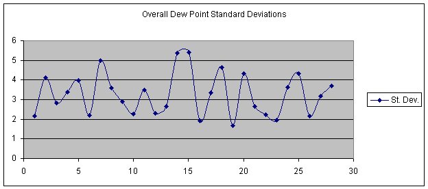
Graph #9
the same cyclic pattern in the plot of overall average errors for each day (Graph #10). One can notice the slight warm bias in the values with noticeable peaks on February 8th and 15th.
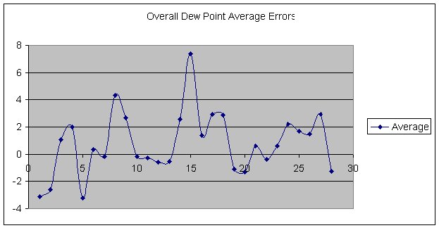
Graph #10
V. Conclusions
V. Conclusions
On average, the MM5 temperature forecasts were colder than verified readings, with February 6th and 10th having significant negative errors. The MM5 dew point temperatures were slightly higher in early forecast periods (00Z-10Z), slightly lower in the mid-range (12Z-20Z), and higher towards the end (23Z-36Z) forecasts. This diurnal oscillation correlates with nighttime and daytime forecast periods, indicating that the model does well around the 11Z and 21-22Z forecasts and has some bias for the other forecast times. Lastly, the Average and Standard Deviation plots show cyclic trends, with the dew point plots having a greater frequency in the oscillation. This oscillation is not diurnal, for the frequency is too high: on the order of 3-5 hours.
Errors have entered our study in a few areas. First, there are gaps in the data where VORTEX did not record data for some reason (most likely due to a lack of communication between the actual station and the remote sensors). While we have adjusted our calculations to not include those data points, they show up on our graphs as zeroes, so it is hard to tell whether the model forecast parameter was correct (zero error) or if there is a missing data point. Typically, if there is a string of zero values, most likely that is a gap in the data. These values can be checked by looking at the data spreadsheet for the particular timeframe in question. Our second source of error is from rounding off all our VORTEX data points for simplicity in our spreadsheets and graphs. Lastly, since all of the verification values were entered by hand into the spreadsheets, there is the possibility that an occasional value could have been rounded off wrong or a wrong time read, yielding the human error element.
VI. Areas for Further Research
VI. Areas for Further Research
While our study has focused on the accuracy of the MM5 Model, there are several questions that can be furthered studied:
1) Why was the model so far off on February 6th and 10th? One could take a closer look at those two days and try to uncover the things that produced the large negative errors in the model temperature forecasts. A look into the other parameters (pressure, winds, etc.) may reveal similar trends.
2) What do the other parameters look like for the month of February? One could see if there are any days that the model was significantly off and if these correlate with the days we observed as being significantly off.
3) Why do the Average and Standard Deviation graphs show a cyclic trend with a frequency on the order of 3-5 hours?
4) Is the diurnal oscillation in the model error the same year round or is this a winter phenomenon, and does this oscillation change with the seasons (i.e. reverse for the summer season)?
Back to top