The Excel Chaos Game
Open an Excel spreadsheet.
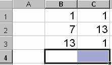
In cells B1, C1, B2, C2, B3 & C3 place the vertices of a triangle, e.g., if you want the
vertices to be (1,1), (7,13) & (13,1) then your six cells would look like:
Next place your “random” point in B4, C4. Choose numbers between 0 and 14 or you
can randomize this too by placing the following formula in both
B4 and C4:
=INT(RAND()*13)+1. Test it by pressing the F9 function key—this causes Excel to
recalculate the spreadsheet & regenerate the random numbers.
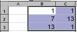
Next highlight cells B1:C3—this is tech talk for click your cursor in cell B1, hold down
the mouse button and drag the cursor to cell C3. The result should look like this:
Click the chart (graph) button,
, and select X,Y (Scatter). Click Finish. Next to the
graph is a key that says Series 1. If you click on it and press Delete (on the keyboard)
you will have more room for the graph. Resize the graph (chart) to fit the space
available. This step will graph the three vertices of your triangle.
Now to include the, “random” point right mouse click the graph and select the option for
Source Data. A dialog box will come up. At this point move the dialog box out of the
way and highlight B1:C4 and click OK. This will now graph the triangle vertices and the
random point.
Click in Cell A5 and type the formula
*
: =INT(RAND()*3)+1. This will generate a
random 1, 2 or 3. It’s just like rolling a three faced die! Continually pressing the F9 key
will let you “see” the results.
Click in Cell B5 and type the following formula
*
:
=(B$1+B4)/2*($A5=1)+(B$2+B4)/2*($A5=2)+(B$3+B4)/2*($A5=3)
Copy and paste this formula into Cell C5.
Highlight cells A5:C5. Grab the little square at in the lower right of C5 and carefully
drag that square down 10 rows to C15. You should now have a series of ones, twos and
threes in Column A and a nice set of decimal ordered pairs in Columns B & C.
Right mouse click the graph and select the option for Source Data. A dialog box will
come up. Move the dialog box out of the way and highlight B1:C15 and click OK. Your
graph should now show 15 points. If you wish to “see” the pattern, right click the graph
and select Chart type. A dialog box will come up. Under Chart Subtype (on the right)
click the third choice down—Scatter with data points connected by lines. Click OK.
This will give you a better visualization of what is happening as you pick points, but after
awhile the lines really get in the way. To remove the lines at this point click the undo
button.
Now highlight A15:C15 and drag the little square in the lower right of C15 down as far
as you dare! Somewhere between 2000 and 7000 rows is okay—I usually use 10,000
+
.
Again right click the graph and select Source Data. Move the dialog box out of the way
and select Columns B & C—this is done by clicking on the B at the top of the column
and holding the mouse button down drag to the C at the top of the next column. Click
OK.
Now you should have a fairly accurate rendition of the Sierpinski’s triangle. If you right
click one of the data points and select Format data series you can “play” with the size and
shape of each data point.
*
About the formulas…
=INT(RAND()*3)+1
RAND() is a built in function that generates a random number
between 0 and 1. Multiplying any result by 3 would generate numbers between 0 and 3.
INT is also a built in function that truncates the decimal part of any number and just
leaves behind the whole number part. Since RAND()*3 leaves us number between 0 and
3, then INT(RAND()*3) leaves us with just a 0, 1, or 2. Since we want 1s, 2s, and 3s, we
add one to each 0, 1, or 2 and we have a formula that works.
=(B$1+B4)/2*($A5=1) + (B$2+B4)/2*($A5=2) + (B$3+B4)/2*($A5=3)
This formula
is a little more complex. (B1+B4)/2 calculates the
12
()
2
+
x
x
part of the midpoint
formula. (The y component is calculated in the C column.)
B1 represents the value of the abscissa of the first vertex, B2 the abscissa of the second,
etc.
The dollar sign represents an absolute cell number—see Excel’s help menu for a
description of relative and absolute references.
A5 contains the value of the die—a one, two or three. Therefore, A5=1 is a truth
statement. If it’s true Excel will return a value of 1, if it’s false a value of 0 is returned.
Therefore, since A5 is a 1, 2 or 3, any particular row, only one of the statements (A5=1),
A5=2) or (A5=3) is true the other two are false. Thereby, multiplying one component of
the formula by 1 and the other two components by 0. Making the sum equal to just one
of the three components.
Back to top